
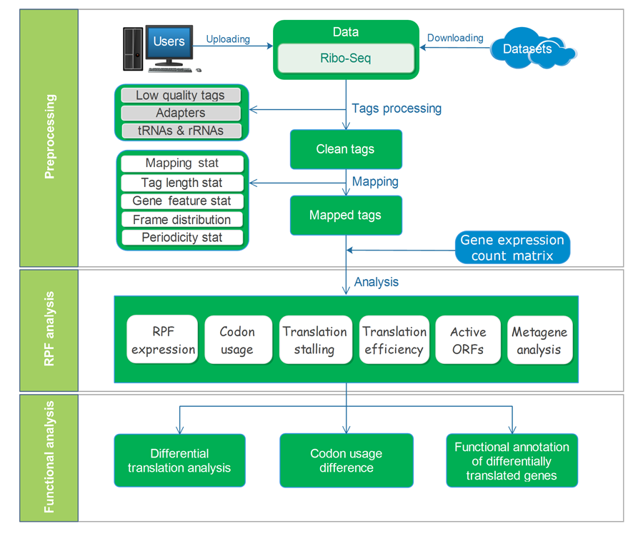
RiboToolkit was constructed based on diverse data sources and tools. tRNA sequences were downloaded from the GtRNAdb database. rRNA and snRNA sequences were retrieved from noncoding RNA annotations in Ensembl Genomes database. Protein coding gene sequences and gene annotations were downloaded from GENCODE for human (V19 and V32 for hg19 and hg38, respectively) and mouse (M23), and Ensembl Genomes database for other species. The overall workflow contains three major parts: (i) Ribo-seq data pre-processing; (ii) RPF mapping and sequences analyses; and (iii) differential translation and functional analyses.
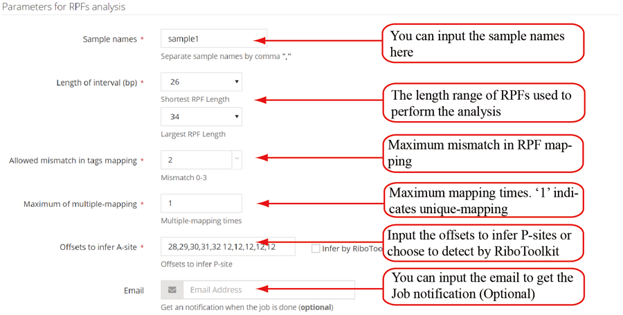
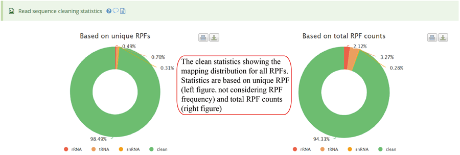
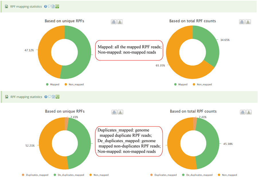
The uploaded sequences were first aligned to rRNAs, tRNA and snRNA to exclude the contaminations using Bowtie v1.2.2 with a maximum of two mismatchs (-v 2) by default. Cleaned RPF sequences were then mapped to the reference genome using STAR v2.7.3a with parameters (--outFilterMismatchNmax 2 --quantMode TranscriptomeSAM GeneCounts --outSAMattributes MD NH --outFilterMultimapNmax 1) by default. The unique genome-mapped RPFs are then mapped against protein coding transcripts using Bowtie v1.2.2 with parameters "-a -v 2" by default. Coding frame distribution and 3-nt periodicity analyses for Ribo-seq quality evaluation are performed based on riboWaltz v1.1.0. The featureCounts program in Subread package v1.6.3 is used to count the number of RPFS uniquely mapped to CDS regions based on genome mapping file (-t CDS -g gene_id), which were then normalized as RPF Per Kilobase per Million mapped RPFs (RPKM). For codon-based analyses, 5’ mapped sites of RPFs (26-32 nt by default) translated in 0-frame were used to infer the P-sites with the offsets, which can be set by users or calculated based on the RPF mapping distribution around translation start sites using psite function in plastid v0.4.8. The codon occupancy was further normalized by the basal occupancy which was calculated as the average occupancy of +1, +2 and +3 position downstream of A-sites. Pause score is further used to evaluate codon pause events using PausePred with default parameters. The upstream and downstream sequences (±50bp) around pause sites were extracted from transcript sequences and different sequences features were calculated, including RNA secondary structure, minimum free energy and GC content. RNA secondary structure and minimum free energy were calculated using RNAfold program in ViennaRNA Package v2.0. For actively translated ORF identification, RPF reads mapped to genome in end-to-end mode were extracted by removing the soft clipped reads from the genome mapping BAM file, then RiboCode v1.2.11, which show high speed and sensitivity for annotating ORF, was used to identify all actively translated ORFs.
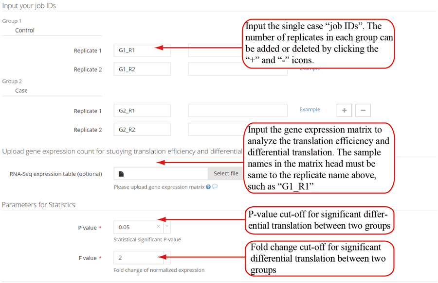
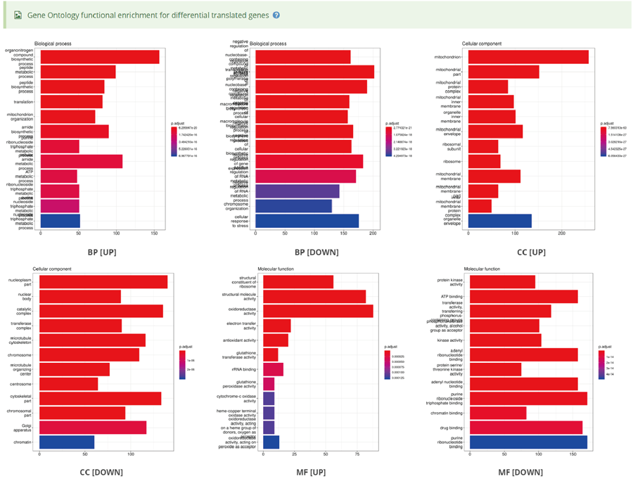
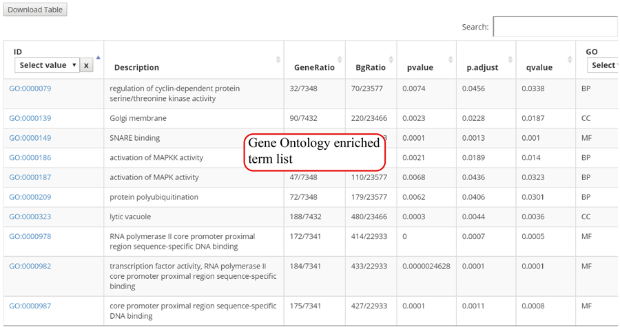
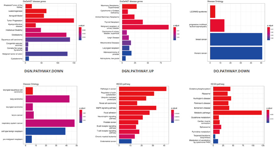
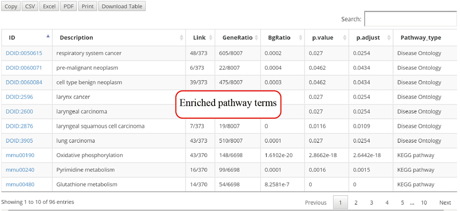
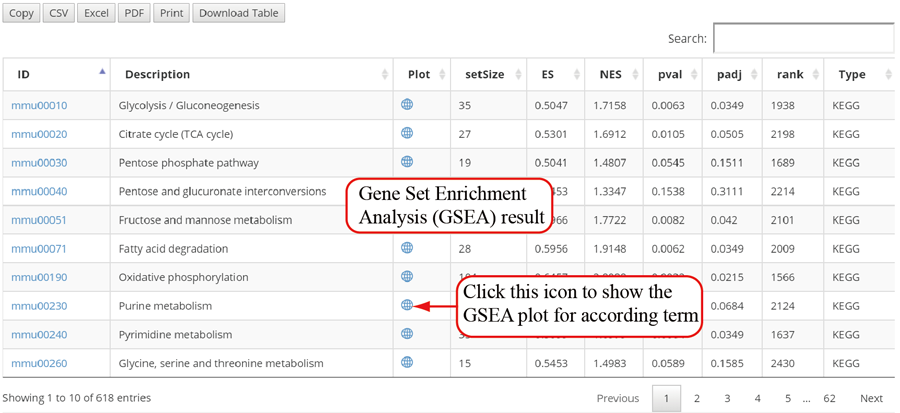
The translation efficiency was calculated as the ratio between CDS RPF abundance and mRNA read abundance for each gene, for which gene expression matrix (read counts) needs to be uploaded by the users in the group case web page. The gene expression count matrix is generated by merging raw read counts from accompanying RNA-seq data for different samples (example commands can be found in next section). RiboToolkit provides the download links of gtf files used for each species. The difference in translation efficiency between two groups with replicates is analyzed using Riborex v2.4.0 (24) based on DESeq2 engine, which models a natural dependence of translation on mRNA levels as a generalized linear model. For two groups without replicates, only fold change is calculated. To explore the biological implication of differentially translated genes (Fold change > 1.5 and adjust p-value < 0.05 by default), various functional gene enrichments are performed, including: (i) Gene Ontology (GO) and KEGG pathway from clusterProfiler package v3.14.3 for all supported species; (ii) Reactome pathway from ReactomePA packages v1.30.0 for human, mouse, rat, zebrafish, fly, and C. elegans; (iii) Disease Ontology, Network of Cancer Gene, DisGeNET disease genes from DOSE packages v3.12.0 for human, mouse, rat, zebrafish, fly, and C. elegans. Meanwhile, Gene Set Enrichment Analysis (GSEA) for GO, KEGG and MSigDB functional gene sets are supported for human, mouse, rat, zebrafish, fly, and C. elegans. In the functional enrichment process, Fisher’s exact test is used to perform enrichment analysis, while for the GSEA analysis, clusterProfiler package is utilized. FDR < 0.05 was set as the significant level by default.
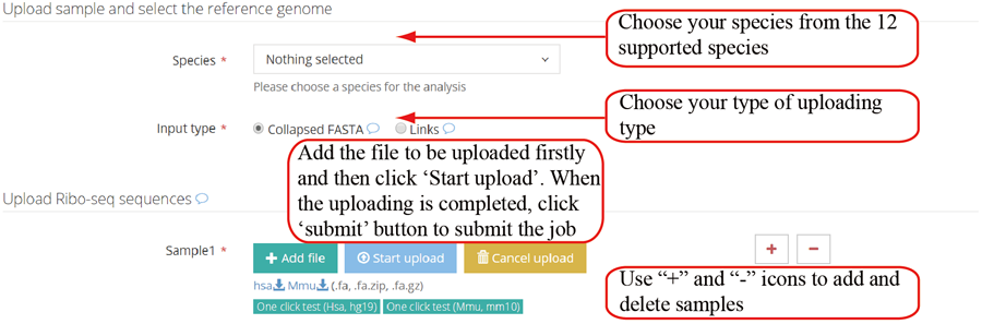
Inputs of single case analysis. RiboToolkit provides the users with two ways to input their data: (1) collapsed FASTA files and (2) web links to their collapsed FASTA files. The files are recommended to be compressed to increase the uploading speed.
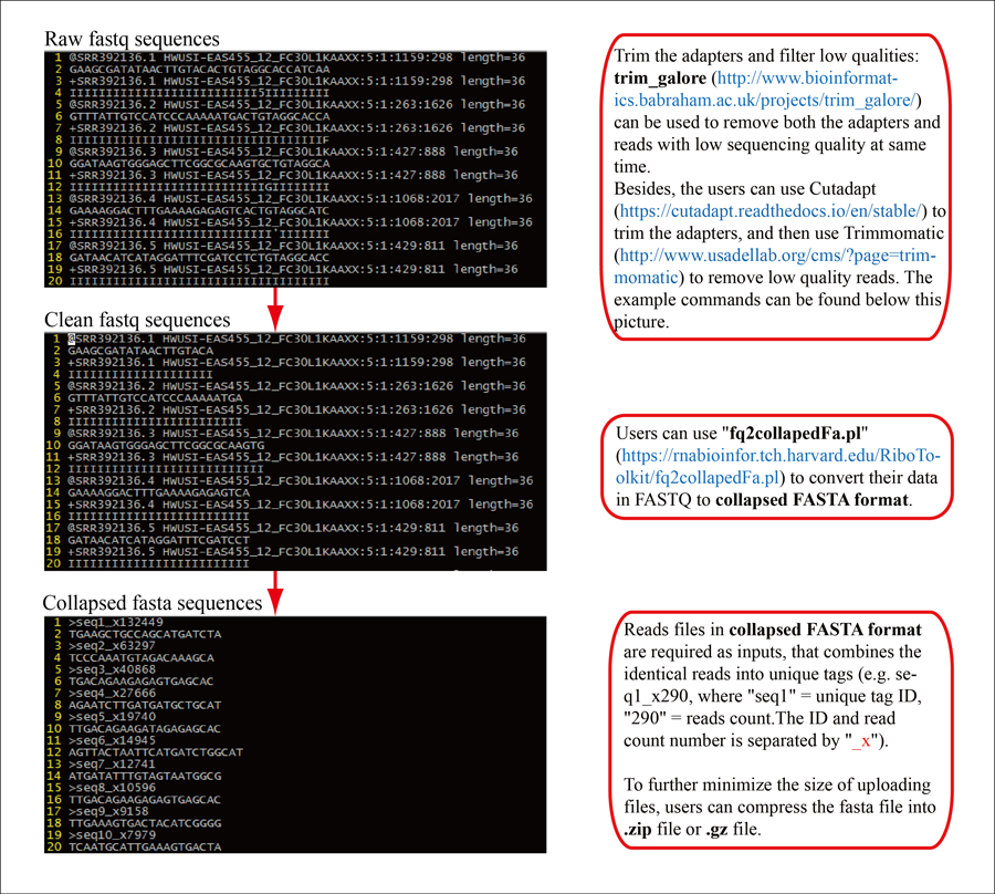
1 Trim adapters and remove low sequencing quality using Cutadapt+Trimmomatic OR trim_galore (example).
cutadapt -a CTGTAGGCACCA --error-rate=0.1 --overlap=3 --times=2 --output=sample.trimed.fastq.gz sample.fastq.gz
-a:3'adapter used in Ribo-seq. The most commonly used 3'adaters for Ribo-seq are: "AGATCGGAAGAG","TGGAATTCTCGG" and "CTGTAGGCACCA".
--error-rate: Maximum allowed error rate as value between 0 and 1 (no. of errors divided by length of matching region) (0.1 = 10%)
--overlap: MINLENGTH Require MINLENGTH overlap between read and adapter for an adapter to be found.
--times: Remove up to COUNT adapters from each read or number of round for adapter finding and removal.
java -jar /path/trimmomatic-0.39.jar SE -phred33 sample.trimed.fastq.gz sample.trimed.cleaned.fastq.gz LEADING:30 TRAILING:30 MINLEN:25
-phred33: Sequence quality type which can be infer using FastQC
LEADING: Cut bases off the start of a read, if below a threshold quality
TRAILING: Cut bases off the end of a read, if below a threshold quality
MINLEN: Drop the read if it is below a specified length
-
trim_galore sample.trimed.fastq.gz --phred33 CTGTAGGCACCATCA --length 25 --max_length 34 -e 0.1 -q 30 --stringency 3 -o outdir
--phred33: Sequence quality type which can be infer using FastQC
--length: Discard reads that became shorter than length INT because of either quality or adapter trimming. A value of '0' effectively disables this behaviour.
-max_length: Cut bases off the end of a read, if below a threshold quality
-e: same as --error-rate in cutadapt
-q: Phred score cut-off
--stringency: same as --overlap in cutadapt
2 Generate collapsed FASTA file.
-i: input cleaned FASTQ sequences (sample_trimmed.fq.gz for trim_galore output)
-o: output collapsed FASTA file
-m: discard reads shorter than minimum length (integer, default: 25)
-l: discard reads longer than maximum length (integer, default: 35)
Download fq2collapedFa_v1.2.pl
Use featureCounts from Subread to generate gene count matrix
featureCounts -t CDS -s 0 -g gene_id -a mm10.annotation.gtf -o sample2.featurecount.txt sample2.bam
featureCounts -t CDS -s 0 -g gene_id -a mm10.annotation.gtf -o sample3.featurecount.txt sample3.bam
featureCounts -t CDS -s 0 -g gene_id -a mm10.annotation.gtf -o sample4.featurecount.txt sample4.bam
paste <(awk '{print $1,"\t",$7}' sample1.featurecount.txt) <(awk '{print $7}' sample2.featurecount.txt) <(awk '{print $7}' sample3.featurecount.txt) <(awk '{print $7}' sample4.featurecount.txt) > all.count.txt
Using htseq-count from HTseq to generate gene count matrix
htseq-count -f bam --stranded no -i gene_id sample2.bam mm10.annotation.gtf > sample2.htseq-count.txt
htseq-count -f bam --stranded no -i gene_id sample3.bam mm10.annotation.gtf > sample3.htseq-count.txt
htseq-count -f bam --stranded no -i gene_id sample4.bam mm10.annotation.gtf > sample4.htseq-count.txt
paste <(awk '{print $1"\t"$2}' sample1.htseq-count.txt) <(awk '{print $2}' sample2.htseq-count.txt) <(awk '{print $2}' sample3.htseq-count.txt) <(awk '{print $2}' sample4.htseq-count.txt) > all.htcount.txt
| Species | Genome version | Source | Example | gene ID |
|---|---|---|---|---|
| Homo sapien | hg19 (gtf file) | GENCODE | ENSG00000185097, ENSG00000230092 | .txt |
| Homo sapien | hg38 (gtf file) | GENCODE | ENSG00000185097, ENSG00000230092 | .txt |
| Mus musculus | mm10 (gtf file) | GENCODE | ENSMUSG00000102693, ENSMUSG00000033813 | .txt |
| Mus musculus | mm39 (gtf file) | GENCODE | ENSMUSG00000102693, ENSMUSG00000064842 | gtf file |
| Rattus norvegicus | rn6 (gtf file) | Ensembl | ENSRNOG00000023659, ENSRNOG00000016381 | .txt |
| Danio rerio | GRCz11 (gtf file) | Ensembl | ENSDARG00000102123, ENSDARG00000098311 | .txt |
| Bos taurus | ARS-UCD1.2 (gtf file) | Ensembl | ENSBTAG00000006648, ENSBTAG00000049697 | gtf file |
| Canis lupus familiaris | ROS Cfam 1.0 (gtf file) | Ensembl | ENSCAFG00845015183, ENSCAFG00845015195 | gtf file |
| Gallus gallus | GRCg7b (gtf file) | Ensembl | ENSGALG00010000711, ENSGALG00010000715 | gtf file |
| Gorilla gorilla | gorGor4 (gtf file) | Ensembl | ENSGGOG00000010861, ENSGGOG00000040578 | gtf file |
| Macaca mulatta | Mmul_10 (gtf file) | Ensembl | ENSMMUG00000023296, ENSMMUG00000036181 | gtf file |
| Pan troglodytes | Pan_tro_3.0 (gtf file) | Ensembl | ENSPTRG00000052463, ENSPTRG00000042737 | gtf file |
| Sus scrofa | Sscrofa11.1 (gtf file) | Ensembl | ENSSSCG00000028996, ENSSSCG00000005267 | gtf file |
| Xenopus tropicalis | UCB Xtro 10.0 (gtf file) | Ensembl | ENSXETG00000045641, ENSXETG00000042394 | gtf file |
| Drosophila melanogaster | Dm6 (gtf file) | Ensembl | FBgn0267430, FBgn0086378 | .txt |
| Caenorhabditis elegans | WBcel235 (gtf file) | Ensembl | WBGene00017080, WBGene00005298 | .txt |
| Saccharomyces cerevisiae | R64 (gtf file) | Ensembl | YDL163W, YDL076C | .txt |
| Anopheles gambiae | AgamP4 (gtf file) | Ensembl | AGAP002473, AGAP001777 | gtf file |
| Arabidopsis thaliana | TAIR10 (gtf file) | Ensembl | AT1G01010, AT1G01020 | .txt |
| Oryza sativa | IRGSP-1.0 (gtf file) | Ensembl | Os01g0100100, Os01g0100300 | .txt |
| Zea mays | B73_RefGen_v4 (gtf file) | Ensembl | Zm00001d027230, Zm00001d027259 | .txt |
| Zea mays | B73 NAM 5.0 (gtf file) | Ensembl | Zm00001eb015280, Zm00001eb000610 | gtf file |
| Glycine max | Wm82.a2 (gtf file) | Ensembl | Zm00001d027230, Zm00001d027259 | .txt |
| Solanum lycopersicum | SL3.0 (gtf file) | Ensembl | Solyc01g005030, Solyc01g005620 | .txt |
| Vitis vinifera | PN40024.v4 (gtf file) | Ensembl | Vitvi18g04695, Vitvi18g00828 | gtf file |
| Triticum aestivum | IWGSC RefSeq 1.0 (gtf file) | Ensembl | TraesCS3B02G271600, TraesCS3B02G001500 | gtf file |
| Sorghum bicolor | NCBIv3 (gtf file) | Ensembl | SORBI_3001G113500, SORBI_3001G533100 | gtf file |
| Solanum tuberosum | SolTub 3.0 (gtf file) | Ensembl | PGSC0003DMG400042058, PGSC0003DMG400042081 | gtf file |
| Populus trichocarpa | Pop_tri_v3 (gtf file) | Ensembl | POPTR_001G146100v3, POPTR_001G078300v3 | gtf file |
| Physcomitrium patens | Phypa_V3 (gtf file) | Ensembl | ENSRNA049990314, ENSRNA049990316 | gtf file |
| Medicago truncatula | MedtrA17 4.0 (gtf file) | Ensembl | MTR_4g073010, MTR_4g028310 | gtf file |
| Gossypium raimondii | Graimondii2_0_v6 (gtf file) | Ensembl | B456_009G035000, B456_009G301200 | gtf file |
| Cucumis sativus | ASM407v2 (gtf file) | Ensembl | Csa_3G732670, Csa_3G889960 | gtf file |
| Chlamydomonas reinhardtii | v5.5 (gtf file) | Ensembl | CHLRE_12g484834v5, CHLRE_12g558353v5 | gtf file |
| Brassica rapa | Brapa 1.0 (gtf file) | Ensembl | Bra027712, Bra031227 | gtf file |
| Brachypodium distachyon | bdi.v3.0 (gtf file) | Ensembl | BRADI_1g14170v3, BRADI_1g53295v3 | gtf file |
| Malus domestica golden | ASM211411v1 (gtf file) | Ensembl | MD15G0021200, MD15G0206200 | gtf file |
| Escherichia coli | K-12 MG1655 (gtf file) | Ensembl | b0001, b0002 | .txt |
| Bacillus subtilis | Strain 168 (gtf file) | Ensembl | BSU00010, EBG00000977999 | .txt |
| Pyrococcus furiosus | DSM 3638 (gtf file) | Ensembl | PF0001, EBG00001119311 | .txt |
| Halobacterium salinarum | NRC1 (gtf file) | Ensembl | VNG_0001H, VNG_0003C | .txt |
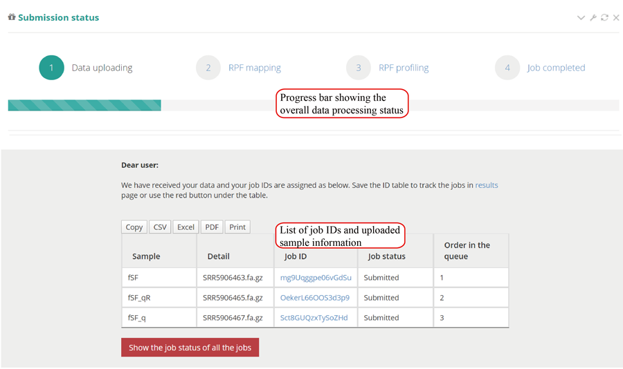
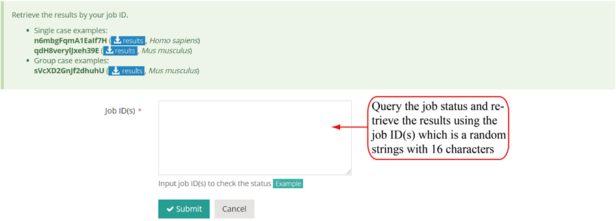
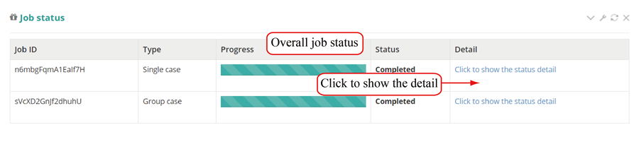
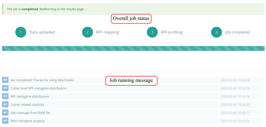
After the job is submitted, the web server will give a table of the Job IDs, which can be used to retrieve the results or perform differential translation analysis in group case study.
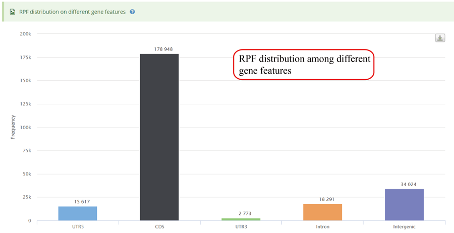
RPFs distribution on different gene features, including 5'UTR (UTR5),CDS, 3'UTR (UTR3), Intron and Integenic region.
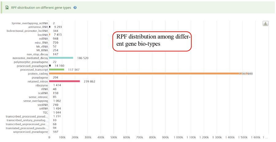
RPF distribution statistics on different gene bio-types, such as protein coding gene, lncRNA and miRNA.
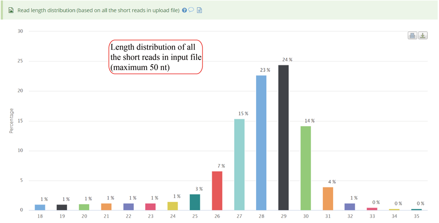
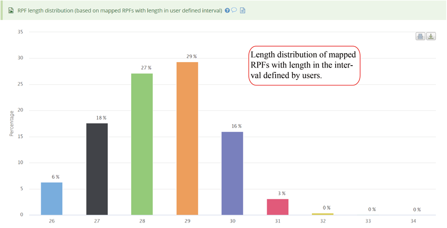
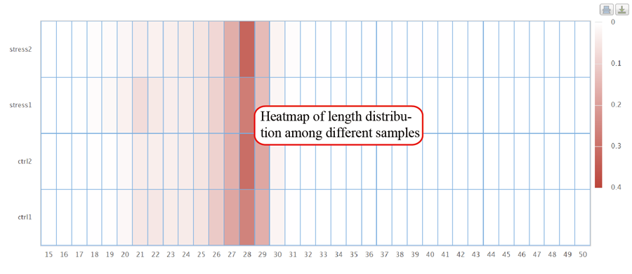
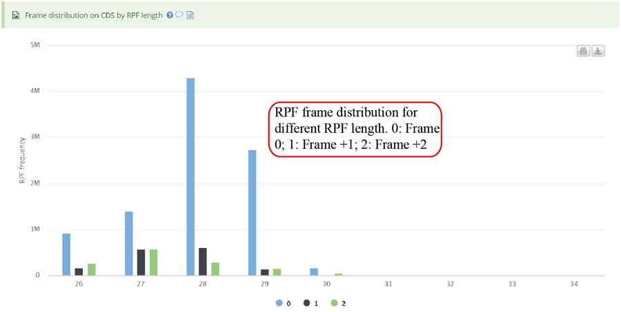
RPF length distribution, which usually peaks at 28 nt or 29 nt in eukaryotic cytosolic ribosomes, reflecting the size of a translating ribosome on the RNA. A broader distribution of reads has been observed in variants of the protocol, depending on the nuclease treatment. Distinct read-length distributions can also correspond to other ribosomal conformations or to ribosomes belonging to different subcellular compartments. Mitochondrial ribosomes have been shown to display a bimodal distribution of read lengths, peaking at 27 and 33 nt, thus showing a clear difference when compared to cytosolic derived RPFs.
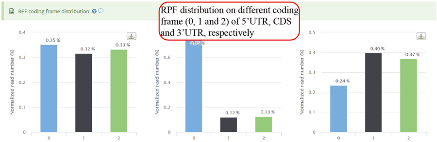
RPFs distribution on different coding frames, including frame 0, frame 1 and frame 2 for 5'UTR, CDS and 3'UTR.
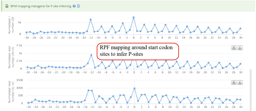
Metagene plot for start codon regions of RPF mapping which can be used to infer P-sites for monosome Ribo-seq.
RPFs periodicity distribution among the translation start codon sites and translation end codon sites.

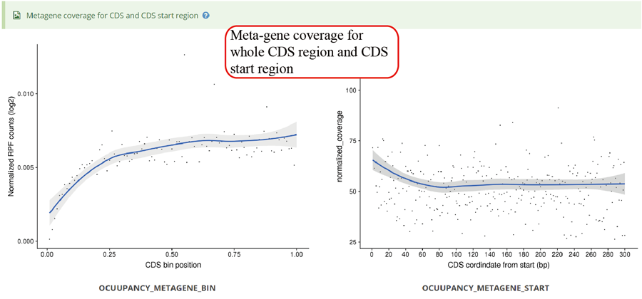
Metagene plot for RPFs on whole CDS region and CDS start regions. The CDS was divided into 100 equal bins.
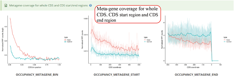
Metagene plot for RPFs on whole CDS region and CDS start regions in group case study. The CDS was divided into 100 equal bins.
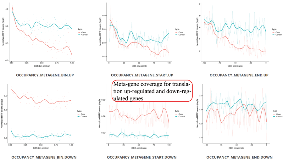
Metagene plot for RPFs on whole CDS region and CDS start regions for differentially translated genes. The CDS was divided into 100 equal bins.
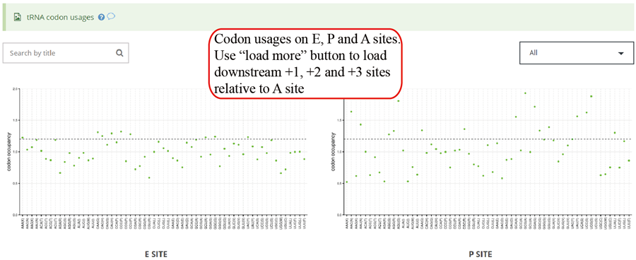
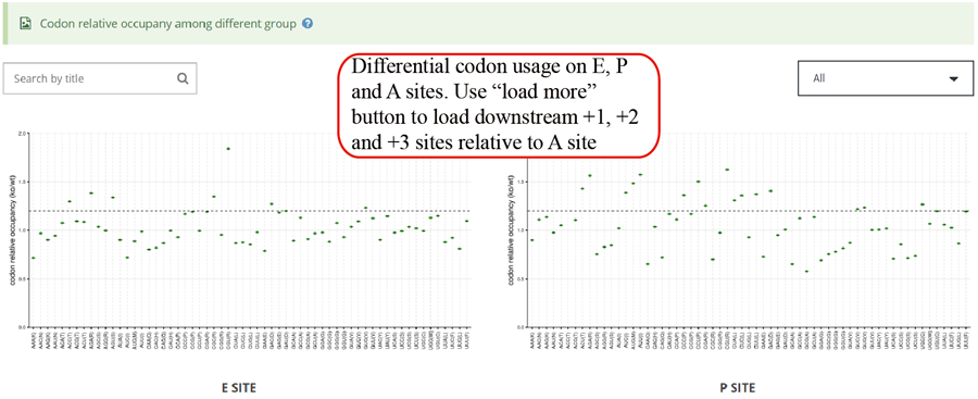
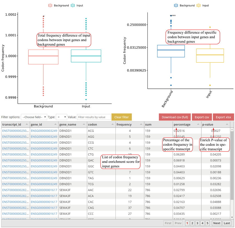
Codon usage on E,P and A sites. The codon usages on +1, +2 and +3 sites relative to A sites will be loaded when users click the 'Load more' button.
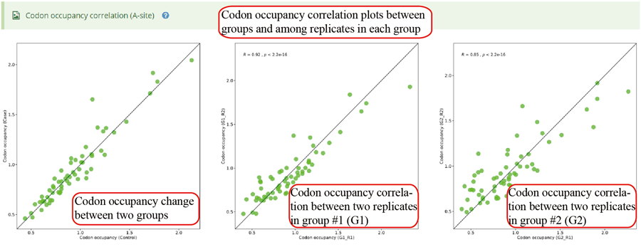
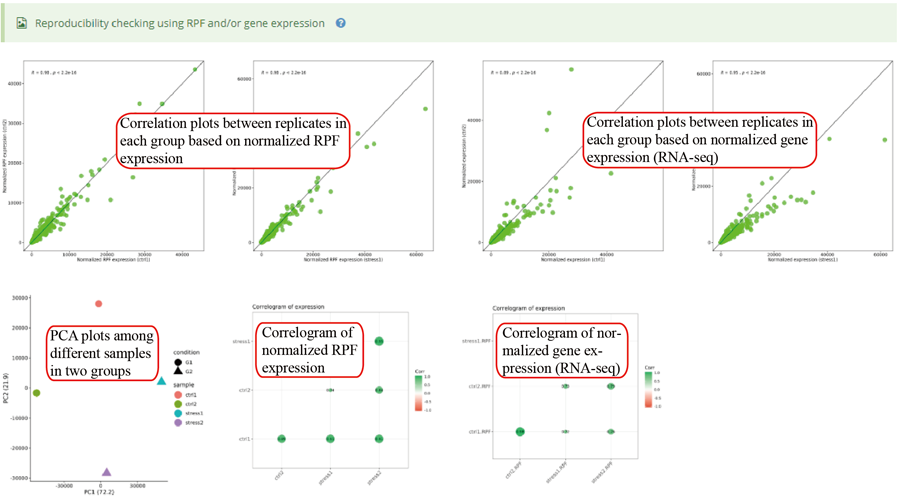
Codon occupancy (A-site) correlation between two groups and among different replicates in each group.
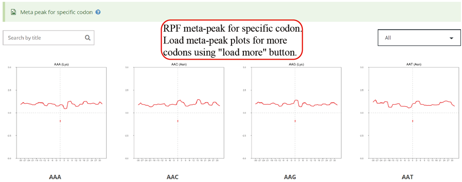
RPF meta distribution on each codon. A sharp peak on the codon indicates that these is a significant stalling on that codon.
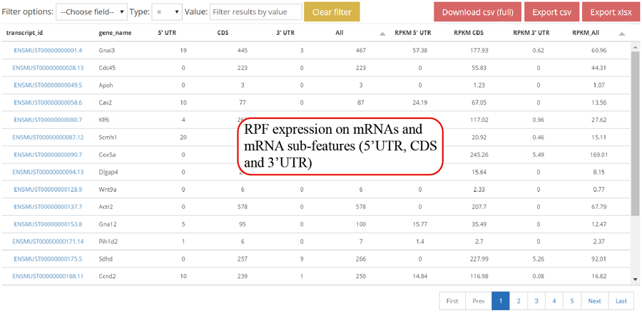
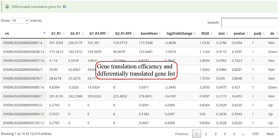
Gene RPF expression values. The RPF expression is calculated for 5'UTR, CDS ,3'UTR and whole mRNA. The raw RPF number and RPKM value are showed.
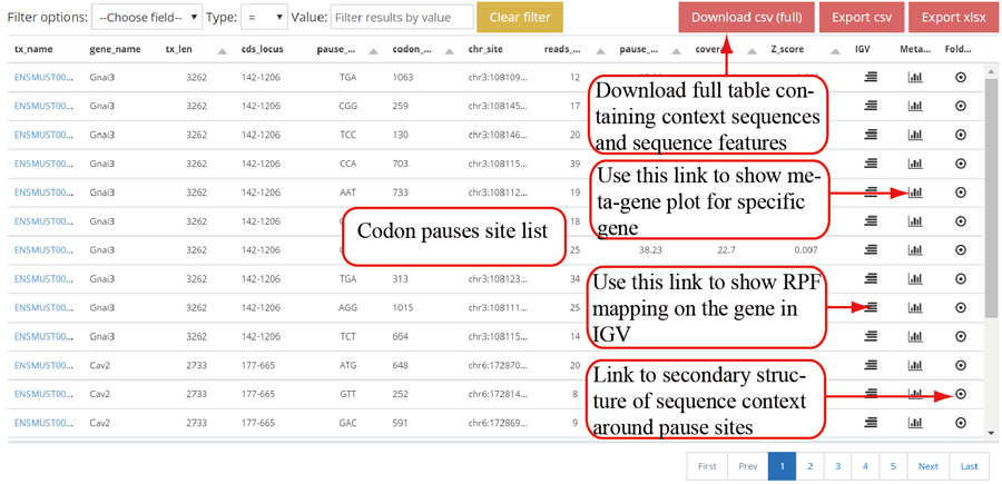
Codon stalling site tables. The more stalling site one gene contains, the more slow translation velocity that gene has. Users can click the icon in peak column to visualize the RPF distribution in IGV.
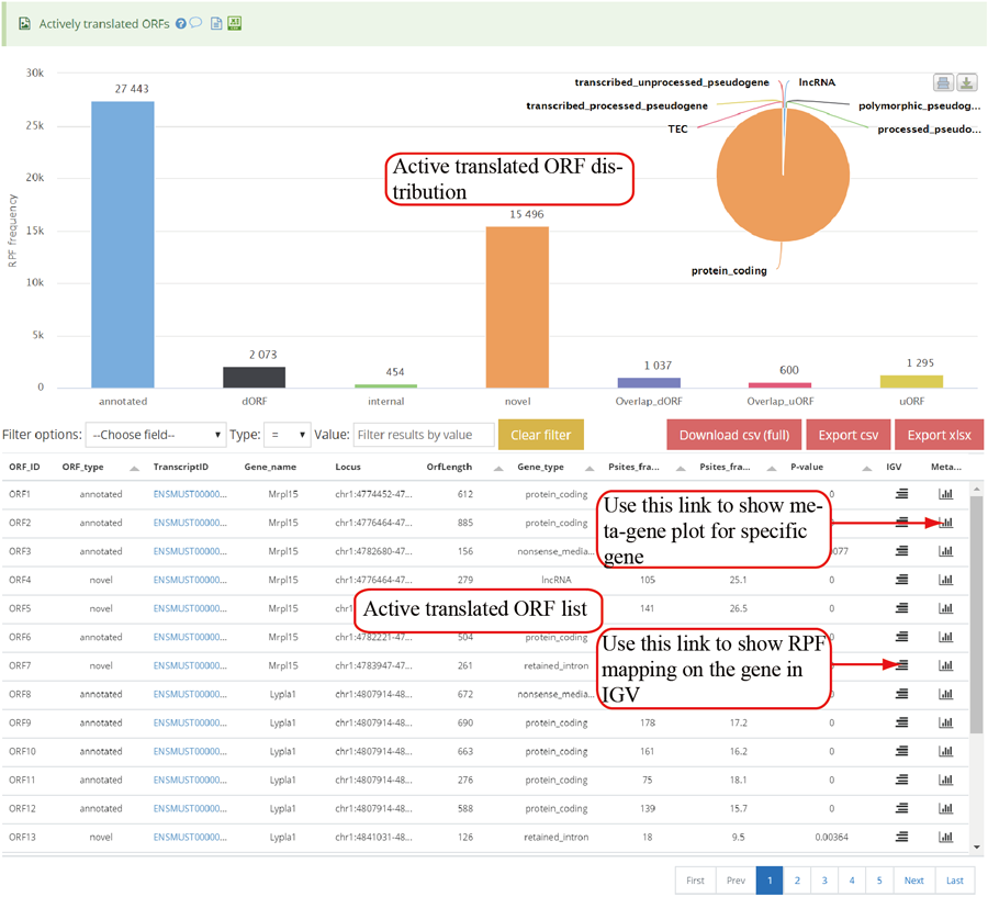
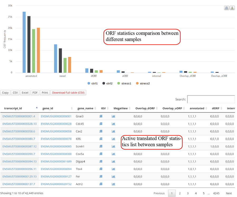
Active translated ORFs. RiboCode was used to call the active translated ORF. The users can click the icon in peak column to visualize the RPF distribution in IGV.
Relative codon usage changes for E, P and A sites in group case comparison study. The relative codon usages on +1, +2 and +3 sites relative to A sites will be loaded when users clicking the 'Load more' button.
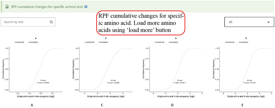
RPF cumulative changes for specific amino acid. Statistics was performed when comparing different groups.
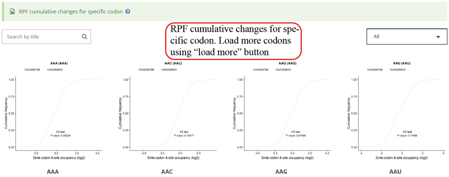
RPF cumulative changes for specific codon. Statistics was performed when comparing different groups.
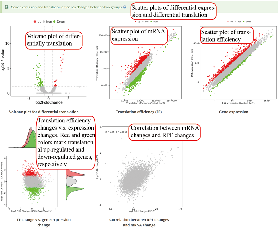
RNA expression and translation efficiency. The pictures use scatter plots to show the differential expression and translation between two groups.

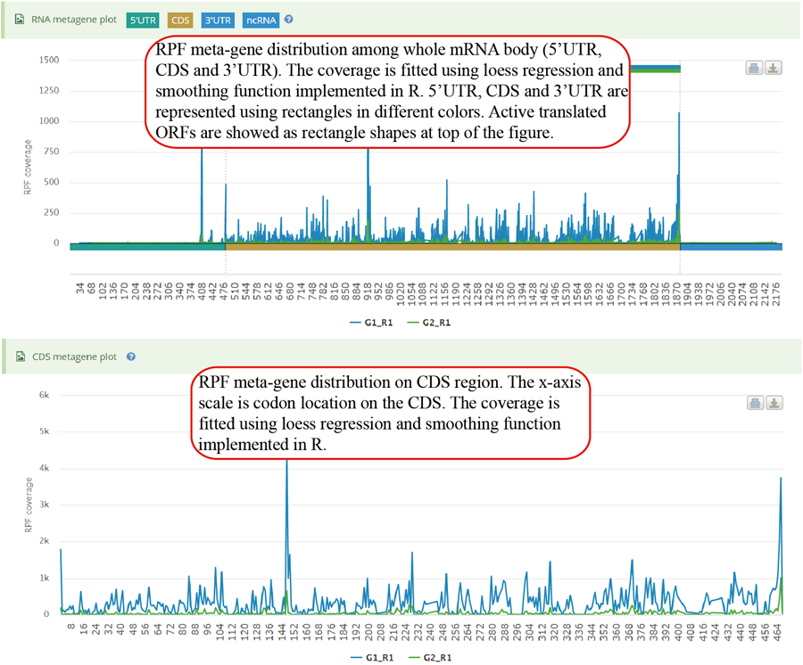
Show the RPF metagene profile for whole transcript and CDS region of specific gene. The RPF coverage is fitted and smoothed using loess regression.
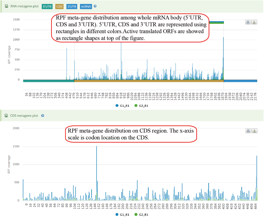
Show the RPF metagene profile for whole transcript and CDS region of specific gene. The RPF coverage is not fitted and smoothed.
| OS | Version | Chrome | Firefox | Microsoft Edge | Safari |
|---|---|---|---|---|---|
| Linux | Centos 7 | 79.0 | 68.3.0 | n/a | n/a |
| MacOS | Catalina | 79.0 | 71.0 | n/a | 13.0 |
| Windows | 10 | 79.0 | 71.0 | 79.0 | n/a |